Mapping raw data to SDTM and ADaM — with the programs written for you.
The mapping usually lives in three places at once: a specification, the programs that implement it, and a Define.xml that describes them. Verdatic keeps one — you confirm the mapping, and the SAS, R and Python come out of it, along with the metadata and the record of every decision.
The problem
Raw data is shaped like the forms it was collected on. SDTM is shaped like the standard. Somebody has to write that translation down, somebody else has to program it, and on the derived side a third person commonly programs it again, independently, to prove the first one right. Then a Define.xml is assembled at the end to describe what the programs did.
- Three artifacts that must agree, and usually don’t. The mapping spec, the program, and the Define.xml are maintained separately. Every change has to be found and landed in all three, and the one that gets missed is discovered by a validator, late.
- The reasoning isn’t written down anywhere. Six months on, nobody remembers why a result came from that field rather than the one next to it — and the person who decided has moved to another study.
- Nothing can be executed until data exists. Programs written against a spec are proven syntactically and hopefully. The real test is first-patient-in, which is also the week nobody has spare.
- Language lock-in. The programs exist in whichever language the group standardized on. Handing the work to a partner who lives in another one means rewriting it.
Risk and cost profile
We don’t publish savings percentages, and there is no benchmark study behind this page. These are the drivers and the units they’re measured in — put your own rates in the last column.
The structural point is simple: most of the cost here is transcription, not judgement. Deciding that a raw field maps to a particular SDTM variable is skilled work. Copying that decision into a spreadsheet, then into a program, then into a Define.xml, then into a QC listing is not — and it is where the errors come from.
| Cost driver | How it shows up | Price it with your own numbers |
|---|---|---|
| Writing it down twice | Once as a mapping specification, again as the program that implements it. | datasets in scope × hours per dataset for spec + program |
| Independent QC programming | Derived datasets are commonly programmed a second time, on purpose, to prove the first. | the QC hours you already budget per dataset |
| Spec, code and metadata drift | Three artifacts that have to agree; each change must land in all of them. | spec revisions per study × the time to propagate one change everywhere |
| Waiting for data | Transformation programs can’t truly be exercised until real records arrive. | weeks between build and first-patient-in — and what your programmers do in them |
| Handover and onboarding | A new programmer reconstructs intent by reading code and asking around. | hours spent answering “why is it mapped that way” per handover |
What we won’t claim: that this removes review, QC or judgement. Generated programs are meant to be read, and every mapping decision is meant to be confirmed by a person. What goes away is the re-typing between spec, code and metadata — they come out of one source, so they can’t quietly disagree.
The workflow, at a glance
The mapping is the artifact. Programs, the Define.xml and the lineage record are all emitted from it, and the official CDISC CORE engine grades what the programs actually produced.
The Verdatic workflow
Real screens from the product, in the order you’d meet them.
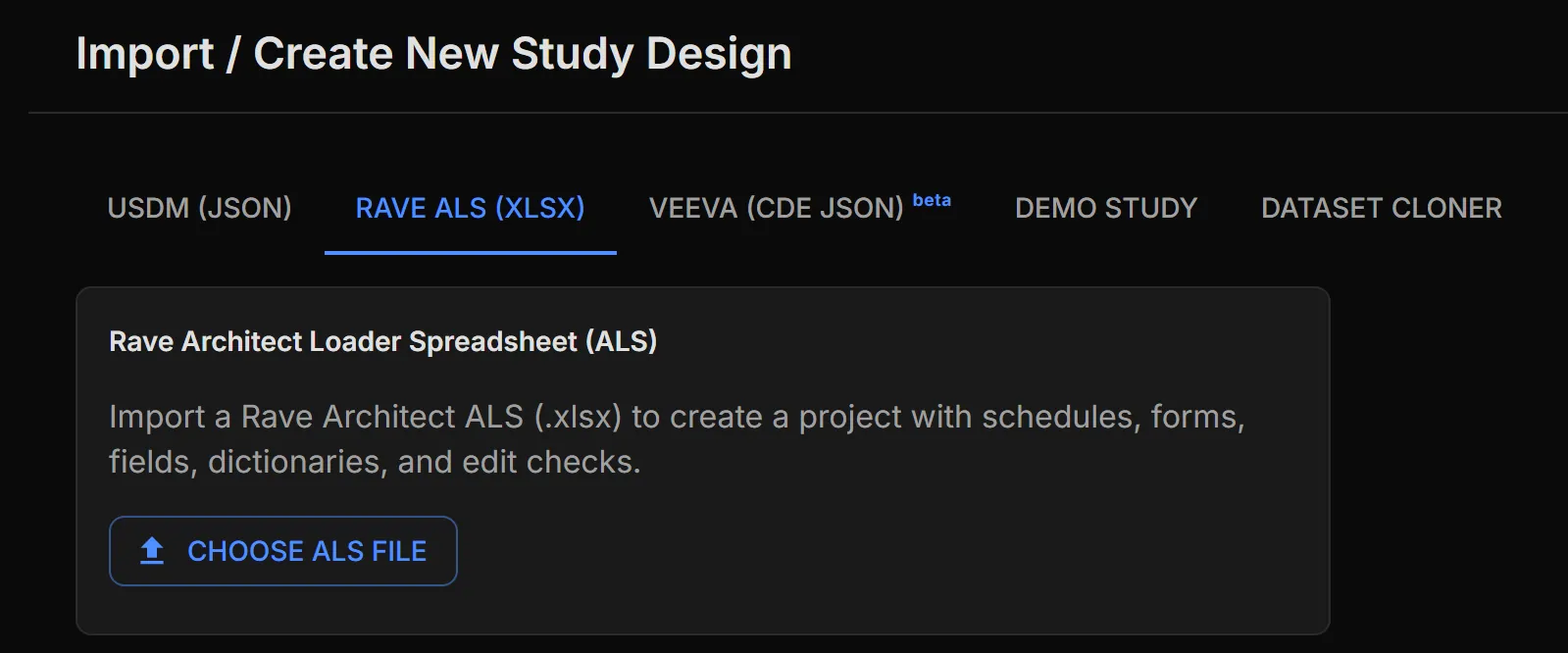
Start from the design you already have
Import a Rave Architect Loader Spreadsheet, a USDM protocol file, or a Veeva casebook design export — or clone the shape of an existing dataset. What arrives is a project with real schedules, forms, fields and dictionaries, which is what the mapping needs to be anchored to.
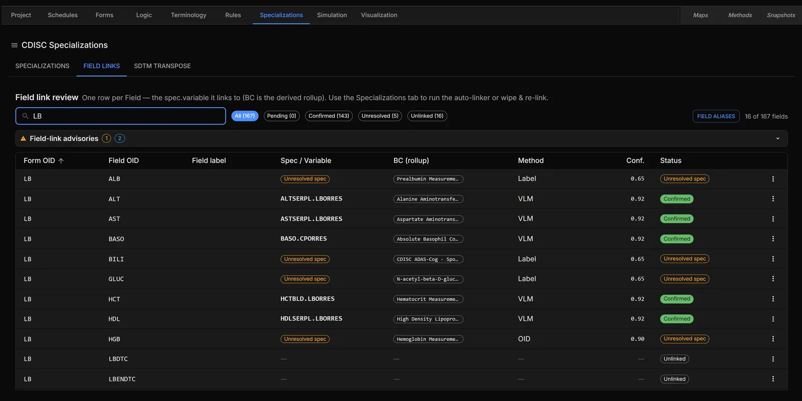
Link each raw field to a standard definition
Verdatic proposes the link between a collected field and the biomedical concept behind it, and shows the confidence and the method that produced each proposal. Strong ones are confirmed; anything uncertain is held back as unresolved for a person to settle. Nothing is silently assumed, and every decision is attributable.
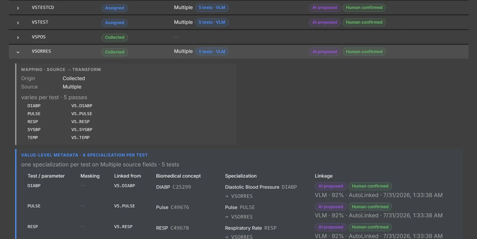
Map to SDTM — and on to the analysis layer
Mapping resolves against a dated snapshot of the CDISC library: biomedical concepts, dataset specializations, controlled terminology and conformance rules, all pinned. The same route continues into the analysis layer, where a subject-level dataset, basic data-structure datasets for findings, and occurrence datasets for events are mapped from the SDTM ones — in dependency order, subject-level first.
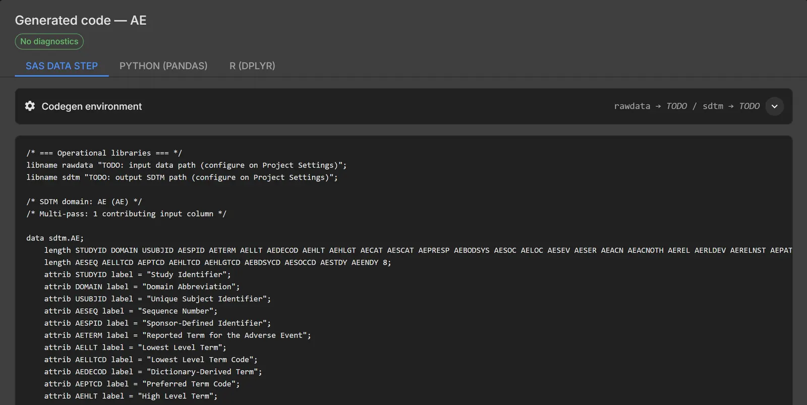
Generate the programs — in all three languages
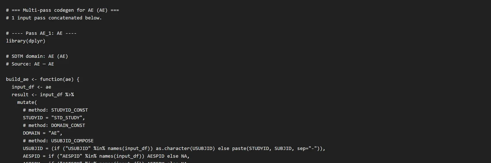
The same mapping emits complete, runnable transformation programs in SAS, R and Python. Same logic, same results, whichever language your team — or your partner’s team — works in. Each derived column carries a comment naming the method behind it, so the program reads as documentation of the mapping rather than as a black box.
Package it so somebody else can run it
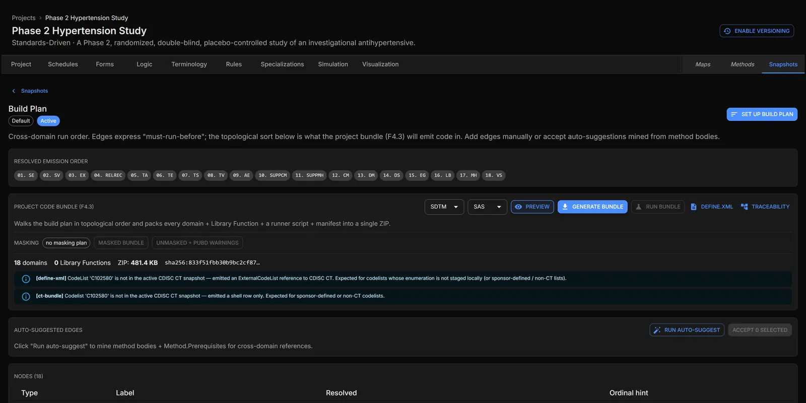
Programs ship as a versioned bundle: a dependency-aware build plan that resolves the order domains must be built in, shared library functions, a Define.xml, and a lineage manifest — checksummed, so the package you hand over is provably the package you built. Analysis datasets are bundled separately from the tabulation ones, each with its own Define.xml.
Run it, and let the official engine grade the result
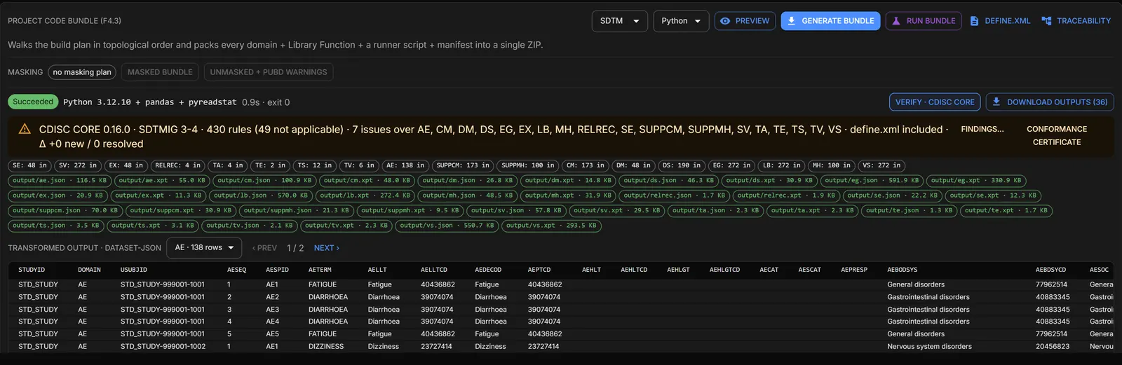
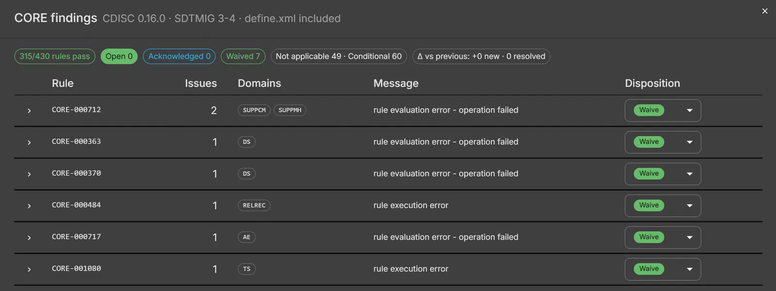
Python and R bundles can be executed without leaving the app, dropping every domain out twice — as a SAS transport file and as Dataset-JSON — and the official CDISC CORE conformance engine checks what the programs produced. Findings become a worklist with a recorded decision on each one and run-over-run deltas, so a resolved issue stays resolved.
Executive summary
- The problem. The mapping lives in three places — a spec, a program and a Define.xml — that must agree and slowly stop agreeing, and none of it can be run until real data arrives.
- The cost. Transcription, not judgement: writing the same decision down repeatedly, QC-programming it a second time, and propagating every change through every artifact.
- What Verdatic does. Proposes each field’s link to a standard definition with a confidence score, keeps the uncertain ones for a person, and treats the confirmed mapping as the single source the rest is generated from.
- What comes out. Runnable SAS, R and Python for the same mapping, a build plan in dependency order, a Define.xml, and a lineage manifest — checksummed and versioned, with tabulation and analysis bundles separated.
- The check. The official CDISC CORE engine grades what the programs produced, and its findings become a worklist with recorded decisions and run-over-run deltas.
Bring us a mapping you already know the answer to.
The most useful first session is a study you’ve already mapped by hand — so you can compare what Verdatic proposes against what your team decided, line by line.
Request accessOr email [email protected]. The CDISC challenge entry follows one measurement through this whole path in six minutes.
The other three use cases